

UY_C59wATYd@outlook.com
New member
- 2021/05/29
- 34
- 17
- 0
2021/05/29
All photos courtesy of the author.
Where Is It?
By Paul Alves, Carmen Wong, Matthew Clampitt, Eric Davis and Eunju Kwak
INNOVATION INSIGHTS with Richard Langley
WE LIVE IN A POLLUTED WORLD. Sometimes even pristine environments are desecrated.
No, I’m not talking here about the rubbish on Mount Everest, nor the leaching of heavy metals from tailing ponds, nor the plastic trash in the oceans, nor the sulfur dioxide in the atmosphere.
I’m talking about radio-frequency pollution. Just as we would like to have our physical environment free of pollution for our better health and that of the ecosystem, we would like the radio spectrum to be free of pollution so that its users — virtually everyone on the planet — can have a better RF experience, whether it be when listening to the radio, using a cell phone or operating a GNSS receiver. We usually call RF pollution interference, or RFI for short, as it interferes with the signal we are trying to receive.
RFI can be accidental or deliberate, in which case we call it jamming. As a shortwave radio enthusiast, I am familiar with both types of RFI. Although the majority of the world’s radio stations attempt to coordinate their broadcasts to ensure that two stations don’t try to beam their signals to a particular area on the same or an adjacent frequency at the same time, it does happen, ruining reception. And if a country doesn’t want its citizens listening to certain foreign radio broadcasts, it might attempt to jam them as the Soviet Union did in the past and as China, North Korea, Cuba and several other countries still do.
In this month’s column, we look at GNSS interference. In many cases, GNSS interference is accidental, with a nearby radio device putting out a signal at a fundamental frequency or a harmonic, which lies within the passband of one of the GNSS frequencies.
It could be intentional, too, and we’ve all heard about GPS jammers including the so-called personal privacy devices that deliberately interfere with GPS signal reception. Is there any way to detect GNSS interference and to find its source so that remedial action can be taken? Yes and yes. A team of authors from NovAtel tell us how.
Interference is a growing concern among GNSS users, particularly in parts of the world where radio frequency transmission is not strictly regulated. Intentional interference and jamming is cheap and relatively easy to obtain in the form of personal privacy devices (PPDs). These devices can sometimes cause unintended interference and jamming to important infrastructure such as an airport. In this article, we describe a method for creating an interference map using the NovAtel OEM7 Interference Tool Kit (ITK). The ITK is capable of detecting and eliminating interference, and can be used to measure the power of a received interferer. When data is collected for an area around a static and continuously operating interference source, it can be used to map out the interference over the affected area. We overview a method for mapping the interference and, using a model of power loss over distance, creating a map of the interferer’s likely position. We also discuss simulated results and three case studies with live (real-data) interference sources from India, Canada and Japan.
NovAtel introduced the ITK in 2016. The ITK’s interference detection provides a list of sources, which includes an estimate of the frequency, bandwidth and power of the measured interference. It also provides the power levels across the entire frequency band of the front end. Either of these can be used as measurements of the received interference power levels. When the power levels for a given frequency are combined from multiple locations, they can be used to estimate the power and location of the interference source. The received power levels can also be combined to estimate the interference power as a function of location. The performance degradation experienced by one receiver at a given interference level can be extrapolated to other receivers at the estimated interference levels.
INTERFERENCE DETECTION
The ITK tools include the ability to visualize the power received across the input frequencies (front-end) bands. This can be used to quickly and easily identify any irregularities in the spectrum. These irregularities could be caused by internal interference, which is interference between electrical components introduced through hardware integration or installation. It can also be caused by external interference, such as by a PPD or other nearby radio transmitter.
The ITK’s detection feature identifies potential interference and provides a list of the interference power, frequency and bandwidth. This makes it easier for integrators to automate responses to potential interference without the need to scan the spectrum themselves. FIGURE 1 shows the received signal power and interference detection threshold for the GPS L1 frequency band. In this case there is no interference detected.
FIGURE 1. Received signal power (blue) and interference detection threshold (red) for L1.
The detection threshold is adjustable. However, if it is set too high, it can cause interference to be undetected; if it is set too low, it can cause false detection. For this example, a fairly low value was chosen because we were willing to manually identify the interference source and ignore any false detection.
The ITK also includes tools to mitigate interference, limiting or eliminating its impact. This includes a high dynamic range mode, which is effective in reducing the impact of interference. If this is not sufficient, then notch or low-pass filters also can be applied to completely cut out parts of the spectrum to neutralize the impact of interference or jamming.
FREE-SPACE LOSS
The mapping algorithm, which will be discussed later, requires a model of the power loss as a function of distance (d) to the transmitter. As the wave spreads from the transmission source, the power is lost according to:
(1)
where Lp (dB) is the power loss in dB, d is the distance in meters, and λ is the wavelength in meters. This equation can be expanded into a function of frequency (f, in Hz) and distance (d, in millimeters). Changing the units in this equation changes the constants.
(2)
For example, if the transmitter is broadcasting at 1.237 GHz, then Equation (2) gives
(3)
This ideal power loss is significantly increased by physical obstructions that are common, such as vehicles, buildings, trees or the terrain type. Different materials can have significantly different impacts on the power loss.
Some researchers have used a precomputed power map and map matching for indoor positioning. This method uses the expected received power to position a receiver. The same algorithm that is used to position the receiver could also be used to position the transmitter.
FIGURE 2 shows the received power as a function of distance that was observed for the Calgary test. There is a large variability in the power, likely due to natural obstructions.
FIGURE 2. Received power as a function of distance from the transmitter.
The equation for the line of best fit of this data is significantly different from Equation (3). This is likely due to the obstructions and limited number of data points. Due to problems with inaccuracies with this data fit, any further power calculations will use Equation (2).
MAPPING THE INTERFERENCE IMPACT
Using a single observation of the received interference power, a profile of the transmit power as a function of location can be created using a power decay curve similar to that shown in Figure 2. If we assume that the transmitter is at a given position and use the decay curve through the observed power, then we can estimate the transmit power at that location. When we do this for multiple locations, a power profile is created. This process is shown in FIGURE 3. When these plotted estimates are connected continuously, then we get a power profile.
FIGURE 3. Received power as a function of distance from the transmitter.
This power profile could pertain to a lower power transmitter that is relatively close to the receiving antenna or could be a stronger transmitter that is farther away. A single transmitter at any location could be responsible for the received power depending on the power of the transmitter.
When additional measurement points are added at different locations, the estimated powers of the transmitter for each individual observation can be combined. The estimated transmit power at some of the potential transmitter locations will match between the observations. For potential interferer locations that are far from the true transmitter location, the observations will conflict with each other.
Creating this type of power profile can be useful for pre-analysis. If we assume that none of the measurement locations can observe the interference, then the received interference must be equal to or less than the noise floor. If we assume that the received interference is at the noise floor, then we can use this profile map to identify the power of any hidden, undetectable transmitters in a region. An interferer may be broadcasting under the noise floor, undetectable at that power and distance. For example, if we want to monitor an area for interference around critical infrastructure, such as an airport, then we can deploy a network of ITK receivers. If no interference is detected, it is still possible for interference to be present if the power level of the transmitter is low enough that it does not reach any of the receivers above the noise floor. This analysis can be used to estimate the minimum detectable interference across the area, and used to determine the receiver network spacing and locations to ensure the minimum detectable interference is immediately detected.
FIGURE 4 shows an example of measurement points from the India case study. It shows the estimated power of a potentially undetectable interference source if no interference is detected anywhere at the measurement points. Lighter colors indicate a higher undetectable interference power. Notice how it is possible to miss a weak interferer that is close or a high-powered interference source that is farther away. This also illustrates how much information we can gather from zero-observation points where interference could not be detected.
FIGURE 4. Locations and power of possibly hidden interference sources that would be undetectable by observation points, shown as blue dots (Map data: Google, DigitalGlobe).
This method could be used to determine the path or spacing of receivers to monitor a region to detect interference at a certain level. With some history added into the model so that the uncertainty increased over time, a single receiver or a fleet of receivers could plan out their routes to monitor for interference.
The estimated interference source power can be used to determine the impact of the interference and give an estimate of the location of the interferer. A single static interferer will be assumed when estimating the location of the interferer using a goodness-of-fit model. A grid is created over the interference area. For each point in the grid, the attenuation (power loss) model is used to calculate the residual between the minimum transmit power and all power measurement points. If the residuals are low for all the observed power locations, then this is the most likely location of the interference transmitter.
FIGURE 5. Example of the goodness of fit for potential transmitter location and power.
FIGURE 5 shows an example of this goodness-of-fit test. The red dot shows the location of a potential transmitter location under test. Using the distance attenuation model, the predicted received power for each of the measurement points is calculated. The difference between the expected received power and the actual received power is an indication that this is not the correct transmitter location. The root-mean-square error of the fit error for all the observed points gives a likelihood that the transmitter is at this location.
SIMULATED RESULTS
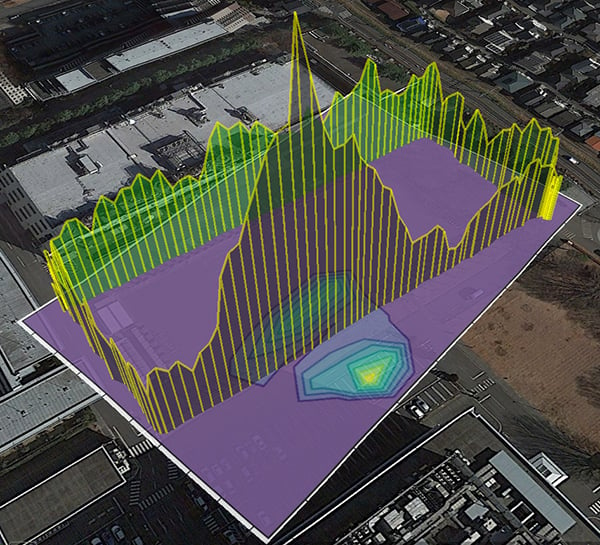
Using the goodness-of-fit method, we can generate reasonable visualizations of the interference effect. FIGURE 6 shows an example map produced from simulated interference to the east.
FIGURE 6. Interference map from a simulation where the interference is on the east side (Map data: Google).
The expected power attenuation model matches perfectly with the data because it is a simulation. Similar results were obtained when the interference was assumed to come from the west and north. The yellow line shows a “roller-coaster” plot of the interference power. The height of the line shows the relative received power. Notice that it increases as we approach the source of the interference and decreases as the path moves away from the interference. A combination of the roller-coaster plot and the map give a quick visualization of the impact and location of the interference. There is a slight ambiguity between the east and west side of the road because the transmitter is close to the road. The goodness of fit works very well in this case to identify the location of the interference source.
FIGURE 7 shows a case where two interference sources are simulated. In this case, the model breaks down because it assumes that there is only a single interference source. The model clearly has difficulties determining the location of the interference. Even with accuracy issues, the model could still be used as a visualization of the interference that is easier to interpret than looking at numbers in a table.
FIGURE 7. Interference map from a simulation with 2 interference sources (Map data: Google).
INDIA DATASET
This dataset was the initial motivation for this work. A customer reported intermittent tracking problems with a newly installed receiver. The receiver would stop tracking for a few hours every evening. Customer service visited the site to investigate. Because of the intermittent nature of the problem, interference was suspected. An OEM729 receiver was walked around the affected antenna in an attempt to find the source of the interference and also to prove to the customer that interference was in fact the cause of the tracking problems.
FIGURE 8 shows the collected measurements. The numbers shown are the received interference powers at each location. It is possible to approximate the location of the interference and the impacted area by looking closely at the measurements, but it takes some close examination and interpretation.
FIGURE 8. Received interference power measured when searching for interference in India.
The source of the interference was identified using this approach. It was found to be a weather station, which performs a nightly upload of data collected throughout the day. This weather station broadcasts at 1580 MHz, which was jamming L1. The customer was able to move the interfering antenna to another site. The customer also could have used the ITK to apply a notch filter, which would have mitigated the interference’s impact, but it is better to remove the source of interference if possible.
Using the data points collected, an interference map can be generated using the method described. This map is shown in FIGURE 9. The lighter color indicates a higher likelihood that the interference transmitter is at that location. The location of the transmitter is also shown in the figure. The likelihood map is very close to the actual location of the transmitter. It gives a quick and easy-to-interpret visualization as opposed to individual measurement points.
FIGURE 9. Interference map for the India case study (Map data: Google, DigitalGlobe).
CALGARY DATASET
We were made aware of a potential unintentional L2 interference device and took it to Cross Iron Mills mall, north of Calgary, Canada, to investigate. FIGURE 10 shows a map of the area.
FIGURE 10. Map of the test area showing the location of the interference source.
We drove the path shown in blue to characterize the interference, and collected data using an OEM729 receiver with the ITK feature. Two buildings are near the interference source: a smaller building to the north and a large building to the south. These buildings block and shield the receiver from the interference when it is between the interference and the receiver.
The interference device was a transmitter to send video from a drone to a monitor, broadcasting at 1.2 GHz with 800 milliwatts. It was purchased online with no warnings about potential impacts it may have on other systems or devices. As recreational drones (and their electronics) become more popular, unintentional jammers and interference sources could become commonplace. We have no continuous monitoring and enforcement for short-range and short-duration unintentional jammers such as this one.
Although many commercial-grade receivers, such as ones common in cell phone and GPS watches, were unaffected because they only operate at L1, the box the device came in also indicates that there is a 1.5-GHz model capable of broadcasting at 2 watts. With 2 watts at 1.5 GHz, GPS L1 would be significantly jammed. This emphasizes the need for interference detection and mitigation. Nothing is stopping recreational hobbyists from accidentally jamming a significant number of users and services.
FIGURE 11 shows the roller-coaster plot of the interference observed during the test. The height of the yellow bars indicates the received power for the L2 interference. The power is generally higher closer to the interference source and decreases as a function of distance; however, there is a lot of deviation. Physical obstructions also cause significant decreases in received power.
FIGURE 11. Observed power of the interference source (yellow) over the test course (Map data: Google, Landsat / Copernicus, DigitalGlobe).
For example, on the north end of the small building, shown on the right side of the figure, the observed interference power drops to almost zero despite being relatively close to the interference source. The large variations in power throughout the southern loop may be due to partial obstructions from parked cars or outcrops of the building. These physical obstructions cause larger decreases in received power than simply moving the antennas away from each other.
Since the interference was only broadcasting on L2, a position is still available through the other GNSS frequencies. The GPS receiver had difficulty tracking GPS L2 signals because of the interference.
FIGURE 12 shows the number of GPS L2 signals tracked. As the receiver approached the interference source, it became more and more difficult to track the L2 signals. As the receiver moved away from the interference, or behind a physical obstruction (like a building), the impact of the interference decreased and the signals were reacquired.
FIGURE 12. Number of L2 satellites tracked (red) over part of the test course (Map data: Google, Landsat / Copernicus, DigitalGlobe).
This shows how a simple device can inadvertently be harmful. Anyone could have purchased this device to transmit video from their recreational drone. Since this device only broadcasts on L2, the GPS of the drone and many nearby devices would have been unaffected, while almost completely jamming and disrupting any dual-frequency receivers nearby.
FIGURE 13 shows the interference goodness-of-fit map from the real data test. The map shows the correct trend, but the peak of the map does not include the actual location of the interference transmitter. This is due to inaccuracies in the power attenuation model. For example, a significant shift to the south is due to the rapid decrease in power when moving behind the north building.
FIGURE 13. Interference map from the real-data test.
When only the southern dataset is considered, we get a more accurate map, one not impacted by the northern building. This is because the attenuation model does not account for obstructions. The performance of this kind of model could be significantly improved with a model that includes the topography and buildings.
Despite the inaccuracy of the map to precisely locate the interference source, these simple model maps give a nice visualization of the interference.
TOKYO REAL DATA RESULTS
We received a report of interference in Tokyo, Japan, and took a receiver there to investigate. FIGURE 14 shows the maximum received power throughout the dataset. The interference around 1570.69 MHz is obvious and easily to identify in the figure.
FIGURE 14. Spectrum power level for the Tokyo dataset.
FIGURE 15 shows the observed power of the interference source when walking around the building. There is a peak in the received power when moving to one side of the building, while the observed power is relatively constant over the other three sides of the building. This strongly suggests that the interference source is along the one side of the building.
FIGURE 15. Observed power of the interference source (yellow) for the Tokyo dataset (Map data: Google, Zenrin).
This figure also shows the estimated goodness-of-fit interference map produced using the algorithm described earlier. The source of the interference could not be conclusively determined; however, we believe that the source was emanating from one of the vehicles in the parking lot.
This real example illustrates how useful this visualization of the observed power is in understanding the nature of the interference, identifying the source and localizing its effect. The interference in this case did not cause a noticeable change in the number of satellites or signals tracked.
CONCLUSIONS
This article showed a creative and useful application of NovAtel’s Interference Tool Kit available as a feature on the OEM7 line of receivers. The ITK can be used to create maps that show the estimated location of an interferer as well as the impact of the interference on other users. We demonstrated this using simulated datasets where the agreement between the simulated and actual loss-of-power models made for overly optimistic results. Three case studies are also shown: The original motivation for this work was a customer-service case in India. The second is a case in Calgary where unintentional interference was being caused by a drone video transmitter. The third dataset from Tokyo was a similar example, where, unfortunately, the true interference source could not be conclusively identified.
The three interference case studies show the importance of interference detection and mitigation because intentional and unintentional interference sources are easy to obtain and are not easily monitored or restricted. In one of these cases, a device that was naively purchased online as a UAV video transmitter ended up jamming GPS L2 in an area of roughly 2,000 square meters. With interference mitigation, it is possible to continue to work and operate in these environments without interruption or significant impact.
ACKNOWLEDGMENTS
The authors thank Bryan Leedham and Saravanan Karuppasamy for sharing their customer stories with us and providing us with the data for the case studies. This article is based on the paper “Interference Likelihood Mapping with Case Studies” presented at ION ITM 2018, the 2018 International Technical Meeting of The Institute of Navigation, Reston, Virginia, Jan. 29–Feb. 1, 2018.
Paul Alves received a Ph.D. from the Department of Geomatics Engineering at the University of Calgary in 2006. He is a principal research engineer in the Applied Research Team at NovAtel Inc. in Calgary, Canada.
Carmen Wong is a geomatics engineer at NovAtel. She received her B.Sc. in geomatics engineering with biomedical specialization from the University of Calgary in 2008.
Matthew Clampitt graduated in 2014 with a B.Sc. in geomatics engineering from the University of Calgary and is now a developer in the Positioning Algorithms Group at NovAtel.
Eric Davis has an undergraduate degree from the University of Calgary, with majors in both astrophysics and physics. He also earned an M.Sc. in physics at the University of Calgary. He joined NovAtel in 2016.
Eunju Kwak received her Ph.D. from the Department of Geomatics Engineering, University of Calgary, in 2013. She is a geomatics engineer at NovAtel.
FURTHER READING
• Authors’ Conference Paper
“Interference Likelihood Mapping with Case Studies” by P. Alves, C. Wong, M. Clampitt, E. Davis and E. Kwak in Proceedings of ION ITM 2018, the 2018 International Technical Meeting of The Institute of Navigation, Reston, Virginia, Jan. 29–Feb. 1, 2018, pp. 467–482.
• GNSS Interference and Jamming Detection
“Interference” by T. Humphreys, Chapter 16 in Springer Handbook of Global Navigation Satellite Systems, edited by P.J.G. Teunissen and O. Montenbruck, published by Springer International Publishing AG, Cham, Switzerland, 2017.
“Demonstrated Interference Detection and Mitigation with a Multi-frequency High Precision Receiver” by F. Gao and S. Kennedy in Proceedings of ION GNSS+ 2016, the 29th International Technical Meeting of the Satellite Division of The Institute of Navigation, Portland, Oregon, Sept. 12–16, 2016, pp. 159–170.
“Signal Acquisition and Tracking of Chirp-Style GPS Jammers” by R.H. Mitch, M.L. Psiaki, S.P. Powell, and B.W. O’Hanlon in Proceedings of ION GNSS+ 2013, the 26th International Technical Meeting of the Satellite Division of The Institute of Navigation, Nashville, Tennessee, Sept. 16–20, 2013, pp. 2893–2909.
“Know Your Enemy: Signal Characteristics of Civil GPS Jammers” by R.H. Mitch, R.C. Dougherty, M.L. Psiaki, S.P. Powell, B.W. O’Hanlon, J.A. Bhatti and T.E. Humphreys in GPS World, Vol. 23, No. 1, January 2012, pp. 64–72.
Modern Communications Jamming Principles and Techniques, 2nd ed., by R.A. Poisel, published by Artech House, Boston, Massachusetts, 2011.
“Jamming GPS: Susceptibility of Some Civil GPS Receivers” by B. Forssell and R.B. Olsen in GPS World, Vol. 14, No. 1, January 2003, pp. 54–58.
“A Growing Concern: Radiofrequency Interference and GPS” by F. Butsch in GPS World, Vol. 13, No. 10, October 2002, pp. 40–50.
• Radio Frequency Propagation
Radio Frequency Propagation Made Easy by S. Faruque, SpringerBriefs in Electrical and Computer Engineering, published by Springer International Publishing AG, Cham, Switzerland, 2015.
Propagation Losses Through Common Building Materials: 2.4 GHz vs 5 GHz, Reflection and Transmission Losses Through Common Building Materials by J. Crawford, Technical Report E10589, Magis Networks, Inc., August 2002.
• Localization Based on Signal Power
“Indoor Localization Based on Floor Plans and Power Maps: Non-Line of Sight to Virtual Line of Sight” by J.J. Khalifeh, Z.M. Kassas and S.S. Saab in Proceedings of ION GNSS+ 2015, the 28th International Technical Meeting of the Satellite Division of The Institute of Navigation, Tampa, Florida, Sept. 14–18, 2015, pp. 2291–2300.
Links:
item: Wifi jammer command prompt code , wifi jammer Airdrie 4.8 10 votes